
独立成分分析(Independent Component Analysis, ICA)是一种统计信号处理方法,其目标是从多个观测到的混合信号中分离出统计上相互独立的潜在源信号。常用的例子是“鸡尾酒会问题”:在一个房间内有两个独立的声音源(源信号 S1、S2),而麦克风记录到的是两条混合后的音频(观测信号 X1 和 X2)。ICA 方法通过这些混合信号估计出独立的信号(Ŝ1 和 Ŝ2),从而实现对音源的分离。
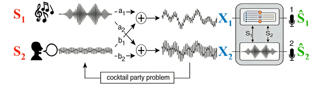
该方法常用于盲源分离问题,通过线性变换将混合数据分解为非高斯、相互独立的成分,广泛应用于语音、图像、脑电图等领域。但需注意的是,由于观测点的信号顺序不确定、信号在观测点的缩放不确定等原因,拆分出的独立信号 Ŝ1 和 Ŝ2 分离结果具有“不唯一性”。因此,分离出的信号并不一定与原始源信号在顺序、符号和幅度上完全一致。
基于数学描述,X1 和 X2 为:
\begin{aligned}
X_1 &= a_1 S_1 + b_1 S_2\\
X_2 &= a_2 S_1 + b_2 S_2
\end{aligned}
即:
\mathbf{X} = A \mathbf{S}, \qquad
\mathbf{X} =
\begin{pmatrix}
X_1 \\
X_2
\end{pmatrix},
\quad
A =
\begin{pmatrix}
a_{11} & a_{12} \\
a_{21} & a_{22}
\end{pmatrix},
\quad
\mathbf{S} =
\begin{pmatrix}
S_1 \\
S_2
\end{pmatrix}
因此,分离独立信号源即:
\hat{\mathbf{S}} = \hat{A}^{-1} \mathbf{X}其可基于 Python 中的 sklearn.decompsition 中的 FastICA 方法快速实现:
import numpy as np
from scipy import signal
import matplotlib.pyplot as plt
from sklearn.decomposition import FastICA

# 混合信号生成参数
np.random.seed(0)
n_samples = 2000
time = np.linspace(0, 8, n_samples)

S1 = np.sin(2 * time) # 信号源 S1
S2 = np.sign(np.sin(3 * time)) # 信号源 S2
S3 = signal.sawtooth(2 * np.pi * time) # 信号源 S3

S = np.c_[S1, S2, S3] # 信号源 S
A = np.array([[1, 1, 1], [0.5, 2, 1.0], [1.5, 1.0, 2.0]]) # 混合矩阵 A
X = np.dot(S, A.T) # 观测信号 X

# 使用 FastICA 进行独立成分分析
model = FastICA(n_components=3) # 设置方法为 ICA
S_hat = model.fit_transform(X) # 计算 S_hat
A_hat = model.mixing_ # 计算 A_hat

# 绘制结果
plt.figure()
plt.rcParams["font.family"] = ["SimHei", "STHeiti"]
plt.subplot(5, 1, 1)
plt.title("源信号 S")
plt.plot(S)

plt.subplot(5, 1, 2)
plt.title("混合矩阵 A")
plt.plot(A)

plt.subplot(5, 1, 3)
plt.title("观测信号 X")
plt.plot(X)

plt.subplot(5, 1, 4)
plt.title("分离信号 S_hat")
plt.plot(S_hat)

plt.subplot(5, 1, 5)
plt.title("分离混合矩阵 A_hat")
plt.plot(A_hat)

plt.tight_layout()
plt.show()得:
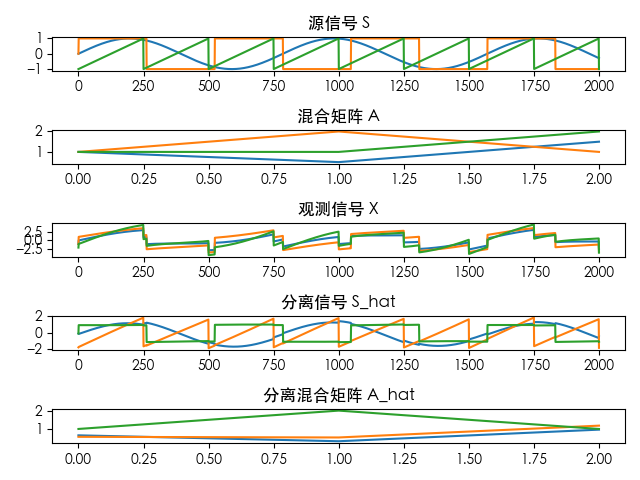
不难发现,与前文所述一致,源信号 S 与分离得到的 Ŝ 在结构形式上保持一致,但其顺序与幅度均可能发生变化。
发表回复